Real-Time Histogram Plots on Unbounded Data

Generating a stream of CPU usage

We first need to generate the data to analyze. We will create items that contain a timestamp and the measured CPU usage every 100ms. We first define a data structure for these items:

CpuMeasure = namedtuple("CpuMeasure", ['timestamp', 'value'])

Then we can emit these items as a stream of data. We use Maki-Nage for this. Maki-Nage is a stream processing framework based on ReactiveX. To generate the source stream, we use ReactiveX directly:

def create_cpu_observable(period=.1):
    return rx.timer(duetime=period, period=period).pipe(
        ops.map(lambda i: CpuMeasure(
            int(datetime.utcnow().timestamp()),
            psutil.cpu_percent()
        ))
    )

The result of this function is a stream object. That is called an observable. This observable emits a CpuMeasure object every 100ms (0.1 seconds).

Plotting and updating a bar-graph

The next step consists in preparing the real-time plot. We want to plot a histogram already computed, so we need a bar-plot. So we use a bokeh vbar widget here. The figure is just initialized, with no data for now.

source_cpu_total = ColumnDataSource(
    data={'edges': [], 'values': []}
)

p_cpu_total = figure(
    title="CPU usage total distribution",
    plot_width=500, plot_height=150
)
p_cpu_total.vbar(
    x='edges', top='values', width=1.0,
    source=source_cpu_total
)

outw = widgets.Output()
display(outw)

with outw:
    h_cpu_total = show(p_cpu_total, notebook_handle=True)

We will later update the plot by setting the source_cpu_total object to other values. The edges field corresponds to the histogram bins, and the value field corresponds to the number of items in each bin.

We can wrap the graph update step in a dedicated function:

def update_histogram(graph_id, source, histogram):
    edges, values = zip(*histogram)
    source.data = {
        'edges': edges,
        'values': values,
    }
    push_notebook(handle=graph_id)

Here graph_id is the bokeh figure object, source the bokeh data source, and histogram the pre-computed histogram.

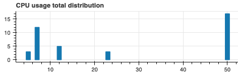
We can test this code by using fake values for now:

update_histogram(
    h_cpu_total, source_cpu_total,
    [(5, 3), (7, 12), (12, 5), (23, 3), (50, 17)]
)

The result looks like this:

Computing the histogram

Now that the data source and the graph are available, we can compute the actual histogram. Maki Nage implements the distribution compression algorithm defined by Ben-Haim et al in the paper A Streaming Parallel Decision Tree Algorithm. That is also the algorithm implemented on the apache Hive histogram_numeric function.

The principle of this algorithm is to compress a data distribution as a dynamic histogram: The bins edges of this histogram are adjusted dynamically as new data come in, but the number of bins is set at creation time. From this compressed representation, one can compute approximations of different metrics with a very good accuracy:

• mean
• variance, standard deviation
• quantiles
• histogram

Since the size of the compressed distribution is fixed, it is very memory efficient and completely independent on the cardinality of the distribution: Whatever the size of the input dataset, you only need 100ths of bytes to compress the distribution!

To fill the compressed distribution we use the math.dist.update operator.

While this compressed representation is a histogram, it cannot be used directly as a displayable histogram: Each bin has unique width, and the number of bins may be much higher than what you want to display. So we use another operator to compute a histogram from the compressed distribution: math.dist.histogram.

The whole computation and display consist of 10 lines of code:

create_cpu_observable().pipe(
    rs.state.with_memory_store(pipeline=rx.pipe(
        rs.ops.map(lambda i: i.value),
        rs.math.dist.update(),
        rs.math.dist.histogram(bin_count=20),
        rs.ops.map(lambda i: (h_cpu_total, source_cpu_total, i))
    )),
).subscribe(
    on_next=lambda i: update_histogram(*i),
)

Let's decompose these lines.

First, we create the observable of CPU usage. Then, we apply a pipe of operations to it. These are data transforms that are applied sequentially to each item. The stateful operations need a state store. That is the location where all intermediate computations are stored. We configure with the with_memory_store operator.

The next step consists in extracting the value of each item. We do not need the timestamp in this first example, so we work on the value field thanks to the map operator.

The two following steps consist in updating the distribution and computing a histogram of 20 bins for each incoming item.

Finally, a tuple is created with the arguments needed to plot the histogram. The histogram is plotted as the sink of this pipeline, in the on_next callback.

Running this code displays a live histogram of the CPU utilization:

Dual monitoring

Now, what if we want to monitor our system since the beginning and also see its recent status (like the last 3 minutes)? We can do this by computing two distributions: A global one, and a recent one on a window of 3 minutes.

To do this we first move the computation to a dedicated function so that we can re-use it:

def compute_histogram(graph_id, source):
    return rx.pipe(
        rs.ops.map(lambda i: i.value),
        rs.math.dist.update(),
        rs.math.dist.histogram(bin_count=20),
        rs.ops.map(lambda i: (graph_id, source, i))
    )

Then we must compute in parallel these two histograms. We use two more operators here.

The first one is the tee_map operator. This operator forwards a source observable to several pipelines so that several computations happen in parallel.

The second one is the split operator. It splits the source observable to windows of 3 minutes. This allows to reset the histogram every three minutes and display only recent data.

disposable = create_cpu_observable().pipe(
    rs.state.with_memory_store(pipeline=rx.pipe(
        rs.ops.tee_map(
            # unbounded distribution
            compute_histogram(h_cpu_total, source_cpu_total),
            # bounded distribution of 3 minutes
            rs.data.split(
                predicate=lambda i:
                    i.timestamp - (i.timestamp % 180),
                pipeline=compute_histogram(
                    h_cpu_recent, source_cpu_recent
                ),
            ),
            join="merge",
        )
    )),
).subscribe(
    on_next=lambda i: update_histogram(*i),
)

With an update on the graph creation, this updates in real-time two histograms.

The whole code of these examples is available here.

Going further

The algorithm presented here is also applicable to distributed systems: The compressed representations of the distributions are mergeable. That is especially useful when you shard a computation on several workers. One can aggregate the final result by merging all partial representations.

It is also possible to use this algorithm in any python environment. The Maki-Nage implementation is in a dedicated package called distogram and has no dependency.

Finally, if you want to learn more about stream processing, you can go through another introduction article I wrote on Maki-Nage.

Originally published in KDnuggets