More and more data science use cases are done in real-time: Alerting, defect detection, prediction, automated recovery are some examples. Yet implementing and deploying them can be very challenging. Maki Nage is a framework that aims at simplifying the development and deployment of real-time processing applications. This article introduces how to use it, showing that stream processing should be simplified!
Addressing The Inference Gap
Before we get our hands on some examples, let me briefly explain why we created Maki Nage. In my DataLab, we often work on real-time streaming services. In practice, the algorithms and machine learning models that we build are fed by Kafka streams. However, the data we use for study and training is retrieved from data lakes. These are batch data, while the inference is running in streaming mode. As a consequence the code that we write for data preparation cannot be used for deployment: We typically use Pandas and Spark to work on batch data, and there is no way to re-use it for deployment. So in the end another team must re-implement the feature engineering part, usually in Java with Kafka Streams.
This situation is quite common in data science and looks like this:
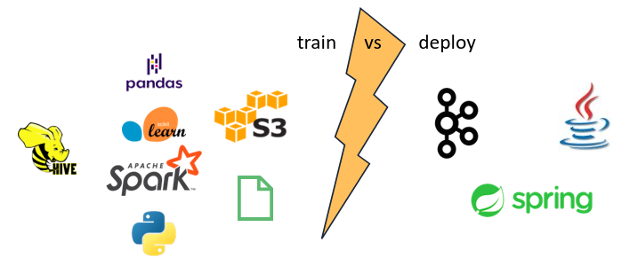
In the end, this double implementation slows down deployment and adds potential bugs due to data not being transformed the same way between training and inference.
Maki Nage aims at reducing this inference gap. It does so the following way:
- Expose a simple and expressive Python API.
- Process batch data in streaming mode.
- Ready to deploy as a Kafka service, with no need for extra infrastructure.
Some tools already exist to do stream processing. But most of them target more developers than data scientists: Kafka Streams, Apache Flink, and RobinHood Faust are such frameworks. Spark Structured Streaming seems to be the exception at the expense of a dedicated cluster.
Maki Nage allows operation teams to deploy code written by data scientists. Still, it supports the whole Python data science stacks.
Now let's dive in!
The First Steps
In this article, we will use the data science library of Maki Nage: RxSci. Installation is done the usual way with pip:
python3 -m pip install rxsci
In the next examples, we will use a list of integers as the source of data:
import rx
import rxsci as rs

source = rx.from_([1, 2, 3, 4, 5, 6, 7, 8])
The from_ operator creates a stream of events from a Python Iterable. In RxSci terms, a stream is called an Observable, and an event is called an Item. These names are from ReactiveX, a building block of Maki Nage.
Here the source Observable consists of a small list, but it could also be a large dataset that would not fit in memory. One great thing with streaming is that one can process datasets much bigger than the available system memory.
Now let's process this data.
Stateless Transforms
The first category of transforms is stateless operations. These are operators where the output depends only on the input item, and no other item received in the past. You probably already know some of them. The map operator is the building block of many transformations. It applies a function on each source item and emits another item with the function applied. Here is how to use it:
source.pipe(
    rs.ops.map(lambda i: i*2)
).subscribe(on_next=print)
2 4 6 8 10 12 14 16
The pipe operator in the first line allows chaining several operations sequentially. In this example, we use only the map operator to double each input item. The subscribe function at the end is the trigger to execute the computation. The RxSci API is lazy, meaning that you first define a computation graph, and then you run it.
Another widely used operator is filter. The filter operator drops items depending on a condition:
source.pipe(
    rs.ops.filter(lambda i: i % 2 == 0)
).subscribe(on_next=print)
2 4 6 8
Stateful Transforms
The second category of transforms is stateful transforms. These are operators where the output depends on the input item and some accumulated state. An example of a stateful operator is sum: Computing a sum depends on the current item's value and the value of all the previously received ones. This is how a sum is computed:
source.pipe(
    rs.state.with_memory_store(rx.pipe(
        rs.math.sum(reduce=True)
    )),
).subscribe(on_next=print)
36
There is an extra step when using stateful transforms: They need a state store to store their accumulated state. As the name implies, the with_memory_store operator creates a memory store. Note also the reduce parameters of the sum operator. The default behavior is to emit the current sum for each input item. Reduce means that we want a value to be emitted only when the source observable completes. Obviously, this makes sense only on non-infinite observables, like batches or windows.
Composition
Things start being great with RxSci when composing all these basic blocks together. Unlike most data-science libraries, an aggregation is not the end of the world: You can use any available operator after an aggregation.
Consider the following example. It first groups items as odd/even. Then, for each group, a windowing of 2 items is applied. Finally, on each of these windows, a sum is computed. This is written in a very expressive way with RxSci:
source.pipe(
    rs.state.with_memory_store(rx.pipe(
        rs.ops.group_by(lambda i: i%2, pipeline=rx.pipe(
            rs.data.roll(window=2, stride=2, pipeline=rx.pipe(
                rs.math.sum(reduce=True),
            )),
        )),
    )),
).subscribe(on_next=print)
4 6 12 14
A Realistic Example
We will end this article with a realistic example: Implementing the feature engineering part for the prediction of the electricity consumption of a house based on weather metrics.
The full example is available in the Maki Nage documentation if you want more details.
The dataset we use is a CSV file. We will use its following columns: atmospheric pressure, wind speed, temperature. The features we want are:
- The temperature.
- The ratio between atmospheric pressure and wind speed.
- The standard deviation of the temperature over a sliding window.
These are simple features. They should be implemented in a few lines of code!
First is some preparation for storing the features and reading the dataset:
Features = namedtuple('Features', [
    'label', 'pspeed_ratio', 'temperature', 'temperature_stddev'
])
epsilon = 1e-5
source = csv.load_from_file(dataset_path, parser)
Then the processing is done in three steps:
features = source.pipe(
    # create partial feature item
    rs.ops.map(lambda i: Features(
        label=i.house_overall,
        pspeed_ratio=i.pressure / (i.wind_speed + epsilon),
        temperature=i.temperature,
        temperature_stddev=0.0,
    )),
    # compute rolling stddev
    rs.state.with_memory_store(rx.pipe(
        rs.data.roll(
            window=60*6, stride=60,
            pipeline=rs.ops.tee_map(
                rx.pipe(rs.ops.last()),
                rx.pipe(
                    rs.ops.map(lambda i: i.temperature),
                    rs.math.stddev(reduce=True),
                ),
            )
        ),
    )),
    # update feature with stddev
    rs.ops.map(lambda i: i[0]._replace(temperature_stddev=i[1])),
)
The first step maps the input rows of the CSV dataset to a Features object. All fields except the standard deviation of the temperature are ready after this operator.
Then a rolling window of 6 hours with a stride of one hour is created. For each window, the standard deviation of the temperature is computed. The last item of each window is then forwarded.
The last step consists of updating the Features object. The tee_map operator used in the second step does several computations on each input item. It outputs a tuple, with one value for each computation branch. Here we have two of them, so two entries in the tuple: The first one is the last feature object for the window, and the second one is the standard deviation of the temperature.
Going further
Hopefully, you should have a good idea of how the Maki Nage APIs look like and how to process time-series with them. Remember from the beginning that one of the aims is to use the same code for training and inference. The last example is the feature engineering phase of a machine learning model. This code can be used as-is to process data from a Kafka stream in production.
Maki Nage contains tools to deploy RxSci code as a service. It also has a model serving tool to deploy models packaged with MlFlow.
Do not hesitate to read the Documentation for more details.
As of writing this article, Maki Nage is still in the alpha stage, but we do not expect significant API changes. We are still working on many aspects of the framework, and you can be involved: Feel free to try it, give some feedback, and contribute!